Verifying empirical rule and Chebyshev's theorem

Empirical rule and Chebyshev’s theorem

Let’s talk about this really simple concept but powerful one. Data Distributions. A data distribution is an abstract concept(a function) that gives the the possible values of data and also how often that data is generated. When you want to talk about the all the data of your experiments at once, then talk about data distribution. A data distribution gives us the probability of how often that data will be an output if we keep repeating the experiment.

We rarely have the complete dataset from the experiment.So, it is powerful to have the an idea of how data is distributed and which data occurs more often than others. We can intuitively understand some distributions like the height of the populations. We know there will be few people with really short height while few have more height. But we are sure that most of the people will be in between.This is really convienient for us to know in advance the spread and frequency of the data.

Interesting thing is that there are more than one kinds of distributions in the world. So the convienience if knowing in advance the spread of the data will be helpful. There is a famous theorem that givrs us an idea of how our data is distributed. It’s called Chebyshev’s theorem.

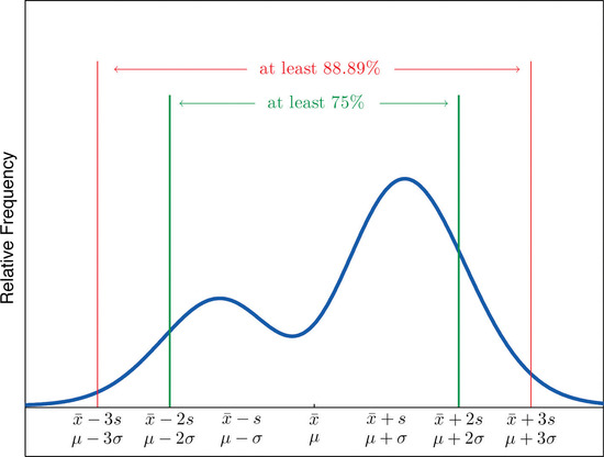
image credit: libretext

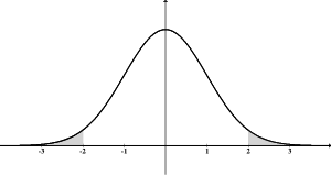
It says that most(3/4th) of our data will be at max two standard deviations from the mean.

library(tidyverse)
library(knitr)
library(kableExtra)
stock<- read.csv("~/OneDrive - MNSCU/FALL 2019/MathStat/Data/Stock Trade.csv",stringsAsFactors = FALSE)

Now let’s clean the name,

stock<- stock %>% select(percentStock = X..of.Shares.Outstanding)

The empirical rule says that 68% of the data will be within two standard deviation.

This function below: 1. standardizes the data
2. counts data within z standard deviations
3. outputs the proportion

data_within<- function(df, z){
  func_normalize<-function(x){(x-mean(x))/sd(x)}
  #>11 after removing a data point 
  df<-df %>% filter(percentStock<11)
  df_scaled<- df %>% mutate(percentStock_normal = func_normalize(percentStock)) %>% filter(abs(percentStock_normal)<z)
  proportion = dim(df_scaled)[1]/dim(df)[1]
  return (round(proportion,2))
}

Let’s collect the output in a small tibble.

tb<- tibble(
  first_std_dev = data_within(stock,1),
  second_std_dev = data_within(stock,2),
  third_std_dev = data_within(stock,3),
)

kable(tb)

We can also test if our function is working correctly,

library(testthat)

## Warning: package 'testthat' was built under R version 3.5.2

normal_generated = tibble(percentStock = rnorm(10,mean = 6.2,sd = 1.2))

#Testing our function
tb_test<- tibble(
  first_std_dev = data_within(normal_generated,1),
  second_std_dev = data_within(normal_generated,2),
  third_std_dev = data_within(normal_generated,3),
)


kable(tb_test)

testthat::expect_gt(tb_test$first_std_dev, 0.68,label = "data proportion within first deivation")

Hence, our function is working correctly.Note that the data is randomly generated every time the code is run.